Deep learning

_{^{4 min read (674 words)}}

Machine learning can be defined as a group of techniques to uncover patterns in data, which can be further helpful to various decision-making tasks [1]. Having the training set pairs in the form of \(\mathcal{D}=\{x_i,y_i\}_{i=1}^N\) where \(N\) is the number of training examples, the task of machine learning model is to identify relationship model between input \(x_i\) and output \(y_i\). Often \(x_i\) is given as an \(D\)-dimensional vector stored in \(N \times D\) matrix \(X\). Here, the input signal \(x_i\) could be of a complex nature: shapes, various structures, time-series data, images, or the features, representing attributes. This setup describes the form of supervised task, which we will focus on further in our thesis. There are, however, other modes of learning [1], unsupervised, self-supervised, and reinforcement, leading to a more generalized and long-term solution in perspective [2].
Inspired by brain connections, called synapses, artificial neural networks (also feedforward neural networks, multilayer perceptron) represent a powerful representation of the learning mechanism. They are the quintessential part of deep learning:

where \(f(\cdot)\) is a nonlinear activation function. Transformed parameters \(\phi_j (x)\) represent group of features characterizing input \(x\). The predicted output also depends on coefficients \([w_j(x)]\) which are updated during training. The different variations of compositions are shown in Figure 1. To learn more complex relationships on more high-dimensional input, deep neural networks have been a viable option in practice. At higher levels of hidden layers, more critical features are transmitted and amplified, whereas less important are restrained.

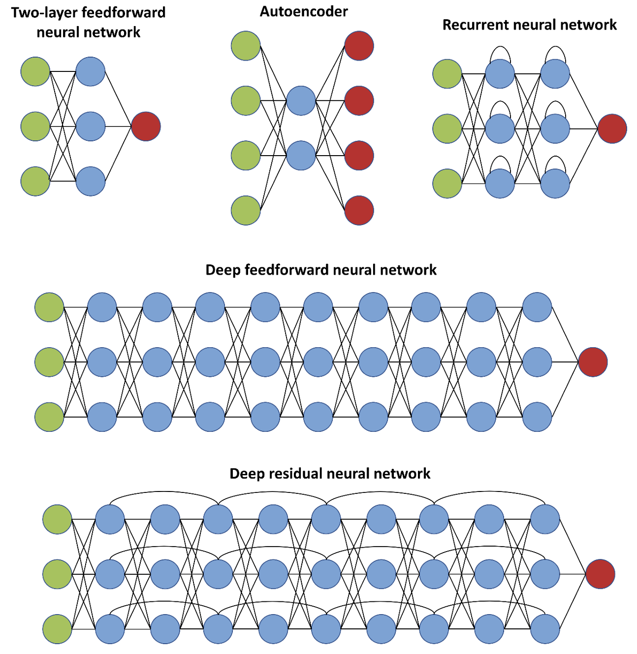
Fig. 1. Architectures of artificial neural networks.

The training of deep neural networks is usually associated with optimization of cost (also value, error) function. Here, the target of the deep learning model is to establish the relationship between the target and predicted based on prior specified function. Dependent on the learning task (classification, segmentation, etc.) cost functions vary, be combinations of multiple, and are still a topic of active research in the community. The most prominent of their representatives could be \(L1\) and \(L2\) familiar with regression tasks. A basic technique of identifying the neural network parameters, for instance, is to minimize a sum-of-squares function. Given the \(x_n\) vectors of input and the target \(t_n\), the objective is minimization of the cost function:

One of the straightforward ways of solving the stated problem is the utilization of gradient information. Gradient descend technique performs weight update in towards negative gradient, therefore:

where \(\eta>0\) parameter represents the adjustable learning rate. This method is trivial and intuitive since it effectively assigns new weight considering the vector to decrease the value of error. This process is repeatedly updated in each iteration until the convergence condition. In practice, more variants of learning strategies are used which could improve speed, and provide more resistance for overcoming local minima. Typical research works report managing these issues by including noise SGD [1], using momentum (Momentum [3], Nesterov [4]), or incorporating adaptive learning rates (Adam [5], Nadam [6]). Additionally, regularization is a common strategy for controlling the complexity of the neural network [7] and generalization.

The concept which gained the most attention in computer vision is a convolutional neural network. Originally this gradient-based learning, proposed in 1998 for digit classification [8], has been long ignored. Only relatively recently in 2012, it helped the team of Krizhevsky to win the ImageNet ILSVRC classification competition, which truly brought a deep learning revolution [9]. In principle, there are four ideas that are combined to contribute to CNN’s success: local connections, shared weights, pooling, and the use of many layers [2].

In a nutshell, the overall layer by layer CNN structure in forward pass can be described as [10]:

\(w\), parameters in layers’ processing, for \(x\), outputs of the previous layer are an input to the next. The convolution function - given the \(V\) data observed: \(V_{i,j,k}\) the value of unit within channel \(i\), at \(j\) row, and \(k\) column as well as \(K\) kernel tensor: \(K_{i,j,k,l}\) showing the connection between a unit in channel \(i\) of output and a unit in channel \(j\) of the input, with \(k\) rows and \(l\) columns offset [11]:

How to cite

Askaruly, S. (2021). Deep learning. Tuttelikz blog: tuttelikz.github.io/blog/2021/09/dl

References

[1] Murphy, K.P., 2012. Machine learning: a probabilistic perspective. MIT press.
[2] LeCun, Y., Bengio, Y. and Hinton, G., 2015. Deep learning. nature, 521(7553), pp.436-444.
[3] Qian, N., 1999. On the momentum term in gradient descent learning algorithms. Neural networks, 12(1), pp.145-151.
[4] Nesterov, Y., 1983. A method for unconstrained convex minimization problem with the rate of convergence O (1/k^ 2). In Doklady an ussr (Vol. 269, pp. 543-547).
[5] Kingma, D.P. and Ba, J., 2014. Adam: A method for stochastic optimization. arXiv preprint arXiv:1412.6980.
[6] Dozat, T., 2016. Incorporating nesterov momentum into adam.
[7] Bishop, C.M. and Nasrabadi, N.M., 2006. Pattern recognition and machine learning (Vol. 4, No. 4, p. 738). New York: springer.
[8] LeCun, Y., Bottou, L., Bengio, Y. and Haffner, P., 1998. Gradient-based learning applied to document recognition. Proceedings of the IEEE, 86(11), pp.2278-2324.
[9] Krizhevsky, A., Sutskever, I. and Hinton, G.E., 2017. Imagenet classification with deep convolutional neural networks. Communications of the ACM, 60(6), pp.84-90.
[10] O’Shea, K. and Nash, R., 2015. An introduction to convolutional neural networks. arXiv preprint arXiv:1511.08458.
[11] Goodfellow, I., Bengio, Y. and Courville, A., 2016. Deep learning. MIT press.