Image classification

_{^{6 min read (1102 words)}}

What is image classification?
Background
Convolutional Neural Networks
A. AlexNet
B. VGG
C. Inception
D. ResNet
How to cite
References

What is image classification?

Image classification is one of the core, non-inverse computer vision tasks on par with segmentation and detection. In the end-to-end learning problem, given the input signal in the form of multiple 2D arrays (mostly RGB: R-red, G-green, B-channels consisting of 3 channels), the objective is to produce a class label from a fixed set of categories. Despite its simple formulation, there are several principal challenges which make this question technically hard. These may include, viewpoint/scale/intra-class variation, deformation, occlusion, etc. Understanding basis of classification from set of classical computer vision will help us more clear translation to the subset of biomedical applications. ˛

Background

Object recognition and image classification task been attacked from multiple angles. Of discriminative nature, several techniques have been proposed as learning classifier for vision: Nearest neighbor (NN, kNN) [1, 2], Neural Networks [3], Support Vector Machines (SVM) [4, 5], Conditional Random Field [6, 7]. These techniques are barely used in practice nowadays due to their inability to learn intricate features of complex, hyperdimensional representations. However, the more fundamental problem is a procedure of handcraftnig features, which are treated into the classifier.

This is a non-automated process, and is always dependent on the expertise of specialist, see Fig. 1.

: Fig. 1. Traditional pattern recognition: a fixed feature extractor and a trainable classifier. Adopted from [8].

Convolutional Neural Networks

Idea of Convolutional Neural Networks with gradient based learning, originally proposed in [8] for digit classification, has been longly ignored. It is with the increase of compute power which helped the team of Krizhevsky, Sutskever and Hinton win the ImageNet competition, which truly brought a deep learning revolution in 2012 [9]. In principle, there are four ideas that are combined to contribute for CNN’s success: local connections, shared weights, pooling and the use of many layers [10].

: Fig. 2. Feature visualization in CNN deep network. Inspired from CS231n.

The learning of a common deep CNN-like architerure occurs as the following. At the input, image is given as a multi-dimensional array of pixels. Each pixel, which is represented between the values \([0, 255]\) is transformed into normalized tensors, an efficient form for gradient computation and further mathematical operations. Convolutional filters, whose weights are initialized randomly in the beginning, have insights after several training iterations at each of the layers. The first layer, typically gains information about edges, their orientations and locations. The second layer could learn about particular arrangements of edges, invariant of type and positions. Further, the third layer, may become aware on isolated parts of the objects. The deeper input travels inside the neural network, the more abstract knowledge we are able to collect. In this way, deep CNNs can learn very complex functions in the end. However, the key idea is that all these features are not handcrafted by the human engineer, but are learnt from data.

The way how layers and blocks of CNN model are organized is named architecture in research papers. These architectures can vary in the number of layers, the depth, the breadth, and the types of additional structures. Each of these engineered blocks are usually suggested to improve classification performance, increase efficiency or to overcome specific issue at the time of their reports.

: Fig. 2. Feature visualization in CNN deep network. Inspired from CS231n.

AlexNet

A revolutional paper in computer vision and deep learning came out in 2012 [9]. Deep convnet, aka AlexNet, was the first to set the path for convnet-based architectures for vision problems. Previously limited by computational amounts of CPU, AlexNet proposed a GPU-based implementation of neural network that made training possible in few days.

The neural network consisited of five convolutional, and three fully-connected layers with 1000-way softwax in the end. Overall, 60 million parameters and 650,000 neurons led to the top performance. The model achieved state-of-the-art performance in ILSVRC-2012 compeitition, in which the objective was to recognize 1000 classes given the unlabelled images. In this paper, novel regularization method, called “dropout” was employed to increase efficiency and learn more robust features.

: Fig. 3. AlexNet

VGG

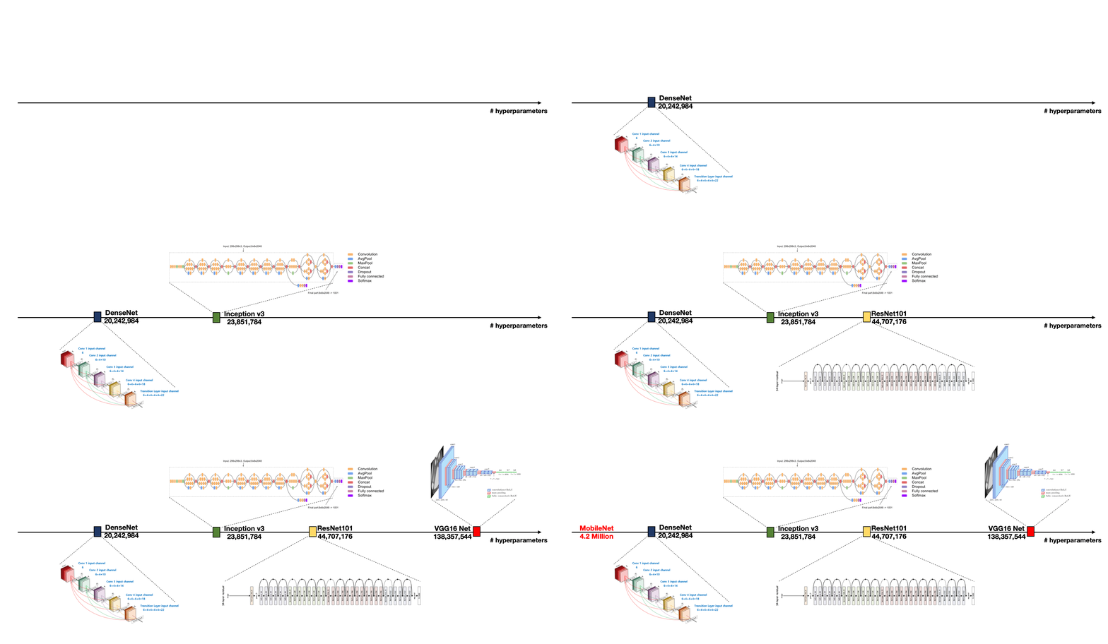
In VGG paper, one more time the focus was put onto the depth of network. The relationship between the number of weight layers and classification accuracy was well studied. It is quantitatively reported that very deep convolutional networks outperform shallow networks. This is due to the increased number of hyperparameters, which make deep architectures able to learn very complex representations.

Particulary configurations for empirical results which were taken: VGG-11, VGG-13, VGG-16, VGG-19, with number specifying the depth of the network. For ImageNet dataset, it was reported that at 19 weight layers, error rate starts to converge. However, with larger gathered datasets, even deeper are expected to further enhance the accuracy. Interestingly, the learnt features can generalize to other tasks and datasets.

: Fig. 4. VGG-16

Inception

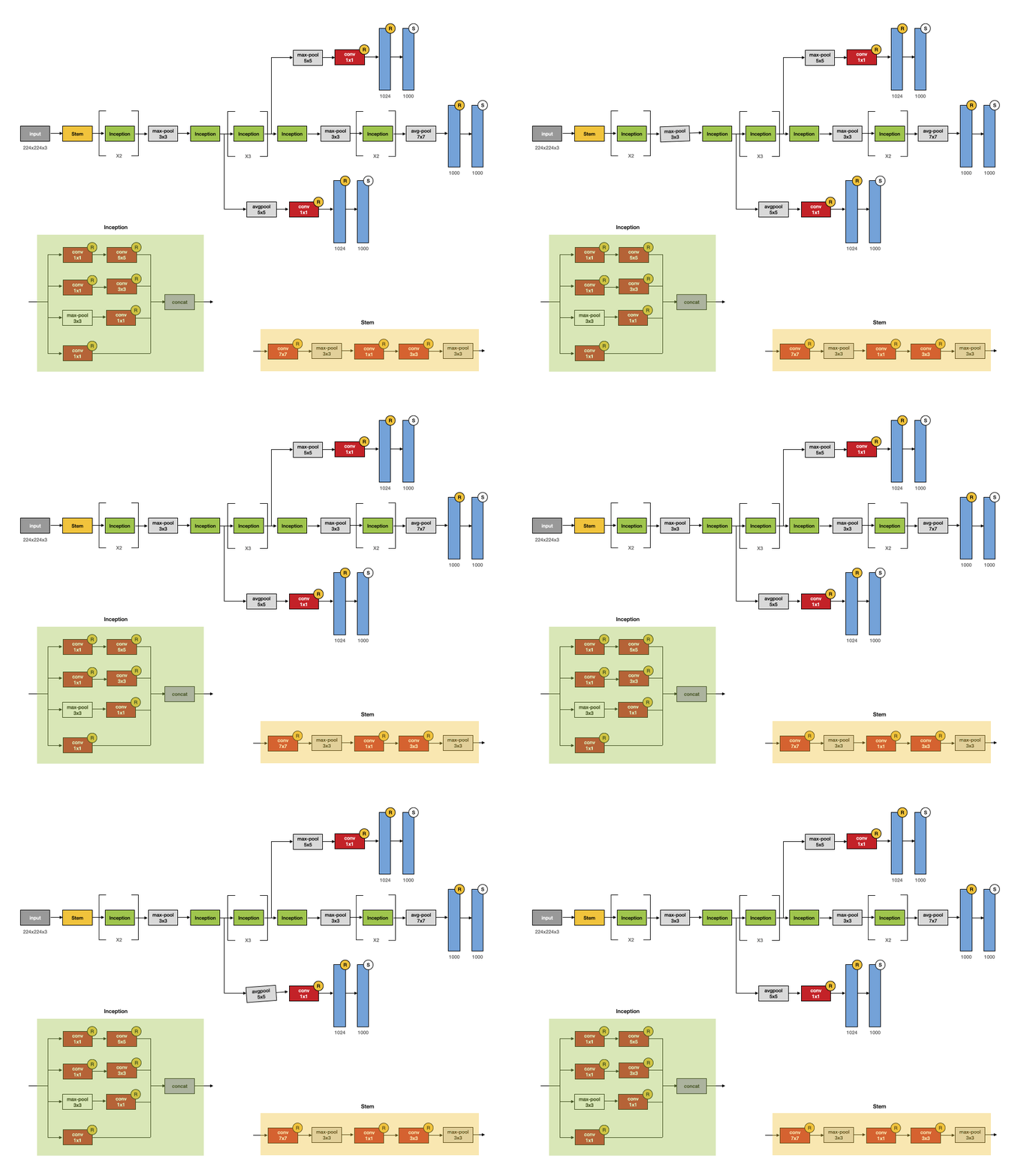
Inception model, suggested in 2014, hallmarks the idea of carefully crafted atchitecture with increased performance. More accurate results has occured due to the more efficient utilization blocks: gradual growth of the network considering both depth as well as width keeping computational budget consistent. Paper mentions building this intuition upon Hebbian principle and multi-scale processing.

22-layer network which contains weights (27 including pooling) set state of the art classification in the ImageNet ILSVRC14. At \(12x\) less fewer parameters than AlexNet, it achieved better classification. The explanation of this, according to the paper, could be related to the two drawbacks caused by substantial number of hyperparameters. The first one is that the larger number of hyperparameters could make neural network more prone to overfit in the absence or proportionally abundant data. Often in practice, gathering high-quality data becomes expensive and non-trivial. Another difficulty is inefficient usage of increased network size. Given the limited amount of compute hardware, it is important to disregard weights which are close to zero, since the number of filter operations to cause them could occupy resources quadratically.

: Fig. 5. Inception V-1

ResNet

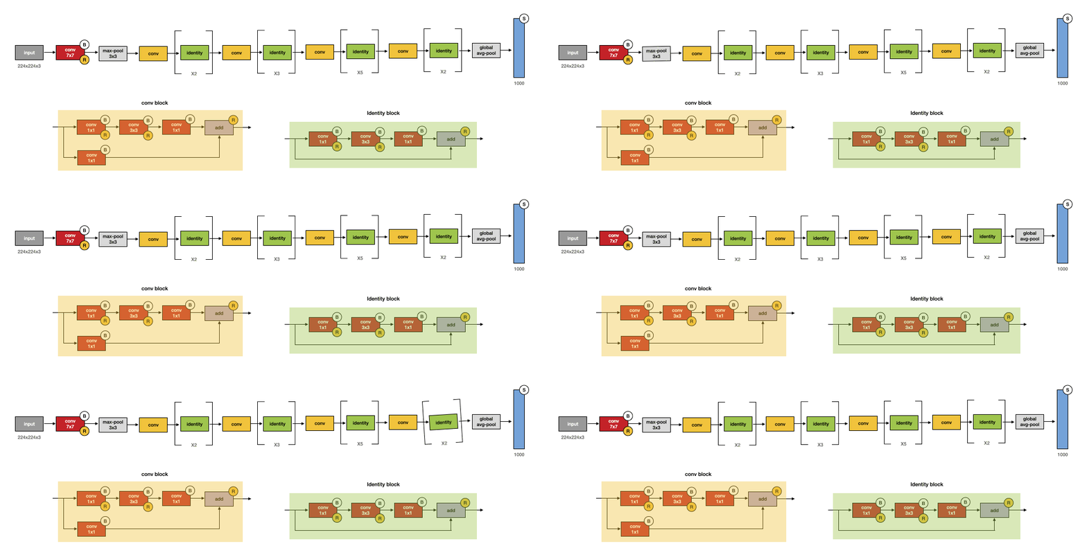
The portion which ResNet architecture is different compared to previous convolutional networks is the ability to stack very deep networks (152 layers). It has been consistently reported previously that deeper networks involve the complex level of features model is able to learn. However, deeper networks are more difficult to train, due to the vanishing gradient (mostly addressed by normalization) and accuracy degradation after saturation (shallower networks learn better than deeper counterparts).
ResNet suggests a residual learning block with identity mapping. In the form of “shortcut connections”, by skipping one or more layers, outputs of previous layer are added to the outputs of stacked layers. Since the identity mapping does not add computational complexity, they are efficient in usage. The residual block prevents degradation problem by giving the network the path to skip extra layers if necesary. This mechanism allowed to set the new state of the art result in 2015. Moreover, this classification architecture is often reused as backbone of extracted features for other computer vision tasks, such as segmentation and detection.

: Fig. 5. ResNet-50

How to cite

Askaruly, S. (2021). Image classification. Tuttelikz blog: tuttelikz.github.io/blog/2021/10/classification

References

[1] Shakhnarovich, G., Darrell, T., & Indyk, P. (2008). Nearest-neighbor methods in learning and vision. IEEE Trans. Neural Networks, 19(2), 377.
[2] Berg, A. C., Berg, T. L., & Malik, J. (2005, June). Shape matching and object recognition using low distortion correspondences. In 2005 IEEE computer society conference on computer vision and pattern recognition (CVPR’05) (Vol. 1, pp. 26-33). IEEE.
[3] Rowley, H. A., Baluja, S., & Kanade, T. (1998). Neural network-based face detection. IEEE Transactions on pattern analysis and machine intelligence, 20(1), 23-38.
[4] Cristianini N., Ricci E. (2008) Support Vector Machines. In: Kao MY. (eds) Encyclopedia of Algorithms. Springer, Boston, MA. https://doi.org/10.1007/978-0-387-30162-4_415
[5] Heisele, B., Serre, T., Pontil, M., Vetter, T., & Poggio, T. A. (2001, January). Categorization by Learning and Combining Object Parts. In NIPS (pp. 1239-1245).
[6] McCallum, A., Freitag, D., & Pereira, F. C. (2000, June). Maximum entropy Markov models for information extraction and segmentation. In Icml (Vol. 17, No. 2000, pp. 591-598).
[7] Kumar, S., & Hebert, M. (2003). Discriminative fields for modeling spatial dependencies in natural images.
[8] LeCun, Y., Bottou, L., Bengio, Y., & Haffner, P. (1998). Gradient-based learning applied to document recognition. Proceedings of the IEEE, 86(11), 2278-2324.
[9] Alex Krizhevsky, Ilya Sutskever, and Geoffrey E. Hinton. 2012. ImageNet classification with deep convolutional neural networks. In Proceedings of the 25th International Conference on Neural Information Processing Systems - Volume 1 (NIPS’12). Curran Associates Inc., Red Hook, NY, USA, 1097–1105.
[10] LeCun, Y., Bengio, Y. & Hinton, G. Deep learning. Nature 521, 436–444 (2015). https://doi.org/10.1038/nature14539

These are suggested materials to proceed with as further readings:

Table of contents